Background
Below, a brief explanation on isosurface construction is given. A more technical description can be found on the excellent website of Paul Bourke.
Isosurfaces are built by picking a single representative value termed the isovalue and finding all points in the domain under consideration which have this value. These points are stitched together to construct a three-dimensional surface.
The construction of isosurfaces, i.e. the set of points that (by approximation) are all associated to the same value of a function, is done using an algorithm called the marching cubes algorithm. In this algorithm, the first step is to define a grid consisting of a set of points on which the function under inspection is being probed. This grid is typically an equidistant grid in three dimensions.
The grid naturally divides the space wherein the function is evaluated into a series of cells wherein each cell contains 8 vertices. For each of the 8 vertices in each cell, it is determined whether the value of the function is larger or smaller than the isovalue. If for one vertex the value is larger than the isovalue and for another vertex the value smaller than the isovalue, then the isosurface has to cut the edge that shares the two vertices. A schematic depiction of this situation is given in Figure 1.
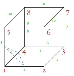
Figure 1: A triangle that is part of an isosurface. For each of the vertices on triangle, the point corresponds to the isovalue. These points lie on the edges 1, 4, and 5 (green numbers) and are found by probing whether the values at the cube vertices 1-2, 1-4, and 1-5, lie on opposite sides of the isovalue.
Given eight vertices per cube, there are only \(2^{8}=256\) possibilities of how a scalar field can interact with each cube. These possibilities are shown in Figure 2. Note that within this set of 256 possibilities, there are only 15 unique results as the majority of the results are linked by a symmetry operation such as a rotation. All these 256 different ways by which the scalar field can interact with each cell are stored in a pre-calculated table by which the resulting list of edge intersections and the polygons that originate from these intersections can be readily found. The exact position where the isosurface intersects each edge is determined using trilinear interpolation.
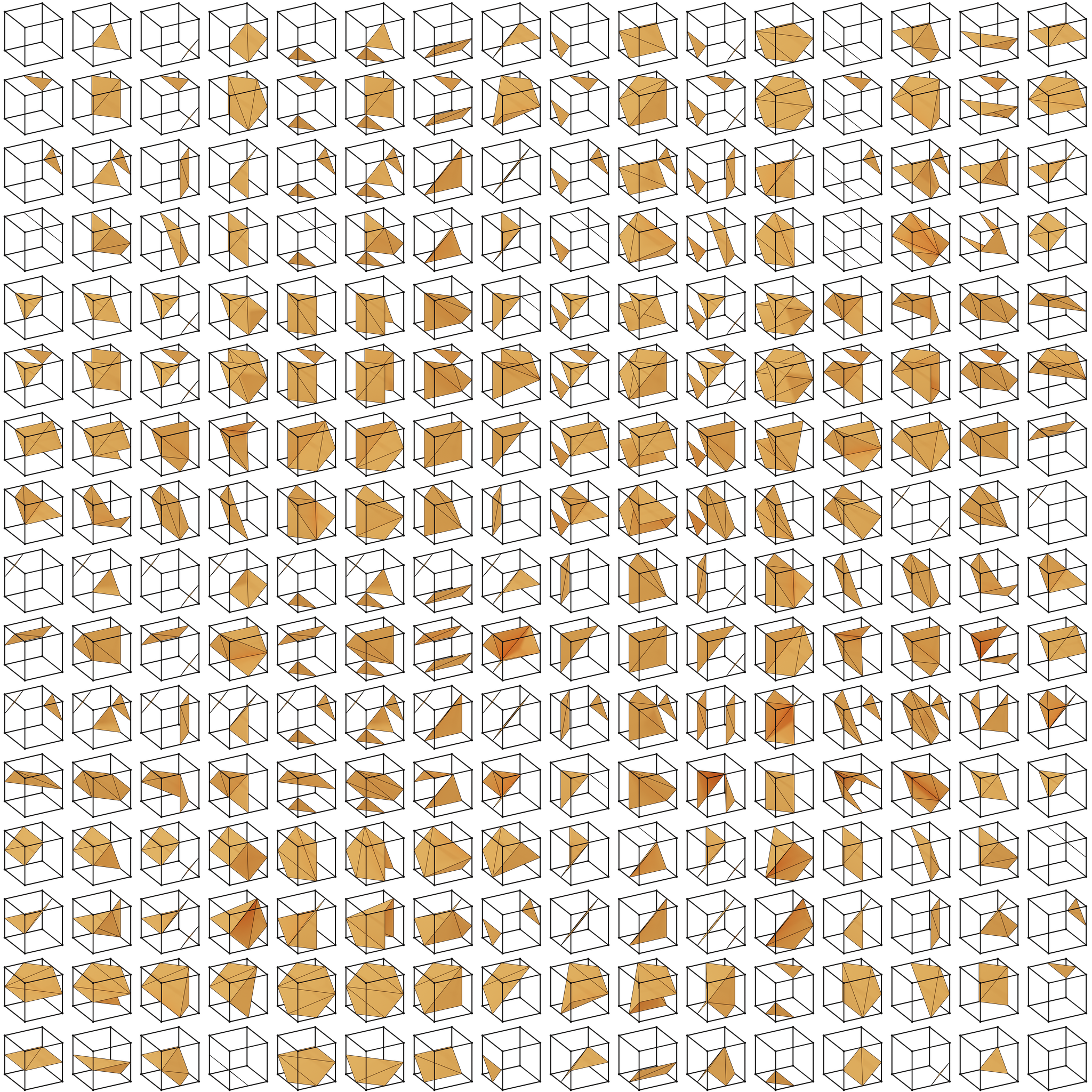
Figure 2: The 256 possible ways that a scalar field can interact with each cube.
Thus the procedure is as follows:
The space wherein the function is evaluated is discretized into small cubes.
For each vertex on these cubes the function is evaluated and it is determined whether the value for the function at each of the vertices is larger or smaller than the isovalue. This leads to a number of edge intersections for each cube from which the polygons (triangles) for each cube can be established.
All polygons are gathered to form the threedimensional isosurface.
It should be noted that this algorithm can be executed in a highly efficient fashion using trivial parallellization as the result for each cube is completely independent from all the other cubes. It turns out that the generation of the scalar field, which by itself is also a highly parallellizable step, is typically the most time-consuming.
The quality of the isosurface depends on the resolution of the grid used to sample the scalar field. The finer the grid (or mesh) used, the better the quality of the isosurface. Thus, rather than using cubes to sample the space, one can use tetrahedra. The algorithm is essentially the same as the one as described above, yet each cube is once more divided into six tetrahedra for which the above algorithm is executed.