Tutorials
This tutorial describes in a step-by-step procedure how to use Den2Obj. Den2Obj comes bundled with a generator to produce scalar fields. As such, no additional calculations on your side are required to follow this tutorial.
Note
To follow along with this tutorial, ensure you have compiled Den2Obj and tested that it is working. See the installation section for more information.
For the visualization of the isosurfaces, we will be making use of Blender. To follow along, please make sure you use Blender 3.3 LTS.
We will not explain how to set materials to objects or how to perform image rendering in Blender. If you are unfamiliar with Blender and wish to learn upon these matters, we can warmly recommend the tutorials by Blender Guru.
Genus2 dataset
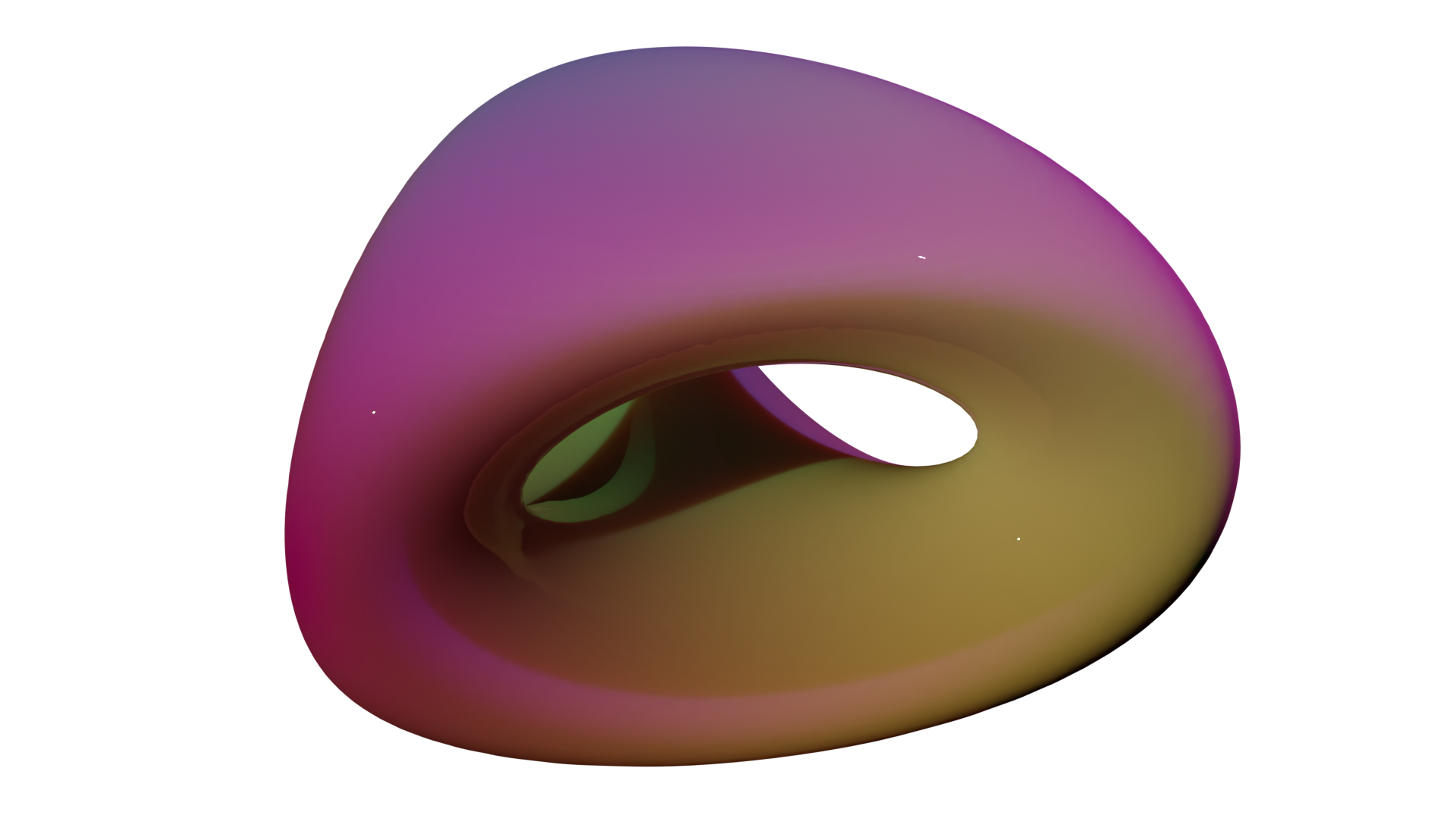
In this tutorial, we will be reproducing the Figure as shown below.
First, we need to build the scalar field. To produce the Genus 2 scalar field, run the following:
./den2obj -g genus2 -o genus2.d2o
You should see the following output:
--------------------------------------------------------------
Executing DEN2OBJ v.1.1.0
Author:  Ivo Filot <i.a.w.filot@tue.nl>
Website: https://den2obj.imc-tue.nl
Github:  https://github.com/ifilot/den2obj
--------------------------------------------------------------
Building grid using dataset: genus2
Looking for best compression algorithm.
Trying GZIP: 2720.5 kb (69.64 %).
Trying LZMA: 1781.2 kb (45.60 %).
Trying BZIP2: 3149.8 kb (80.63 %).
Floating point size determined at: 4 bytes
Writing genus2.d2o (1781.3kb).
-------------------------------------------------------------------------------
Done in 1.42421 seconds.
This will generate a .d2o file containing the Genus 2
scalar field named genus2.d2o. Observe that Den2Obj tests three
different compression algorithms and automatically selects the best algorithm
for the data compression.
To construct the isosurface with an isovalue of 0.1, run:
./den2obj -i genus2.d2o -o genus2.ply -v 0.1 -c
Which will give the following output:
--------------------------------------------------------------
Executing DEN2OBJ v.1.1.0
Author:  Ivo Filot <i.a.w.filot@tue.nl>
Website: https://den2obj.imc-tue.nl
Github:  https://github.com/ifilot/den2obj
--------------------------------------------------------------
Opening genus2.d2o as D2O binary file
Recognizing floating point size: 4 bytes.
Reading 1823992 bytes from file.
Building decompressor
Decompressed data
Done reading D2O binary file
Read 1000000 values.
Using isovalue: 0.1
Lowest value in scalar field: -1.85503
Highest value in scalar field: 265
Identified 48900 faces.
Calculating normal vectors using two-point stencil
Writing mesh as Standford Triangle Format file (.ply).
Writing as Stanford (.ply) file: genus2.ply (1196.8kb).
-------------------------------------------------------------------------------
Done in 0.17653 seconds.
Note
Observe that we generate the isosurface using the -c directive, which
centers the isosurface at the origin. The scalar field is generated in a
cubic unit cell with edges of length 4. If we would not center the object
at the origin, it would be located at position (2,2,2).
Open Blender, remove the original cube and import the genus2.ply via
the drop-down menu as follows:
File > Import > Stanford (.ply)
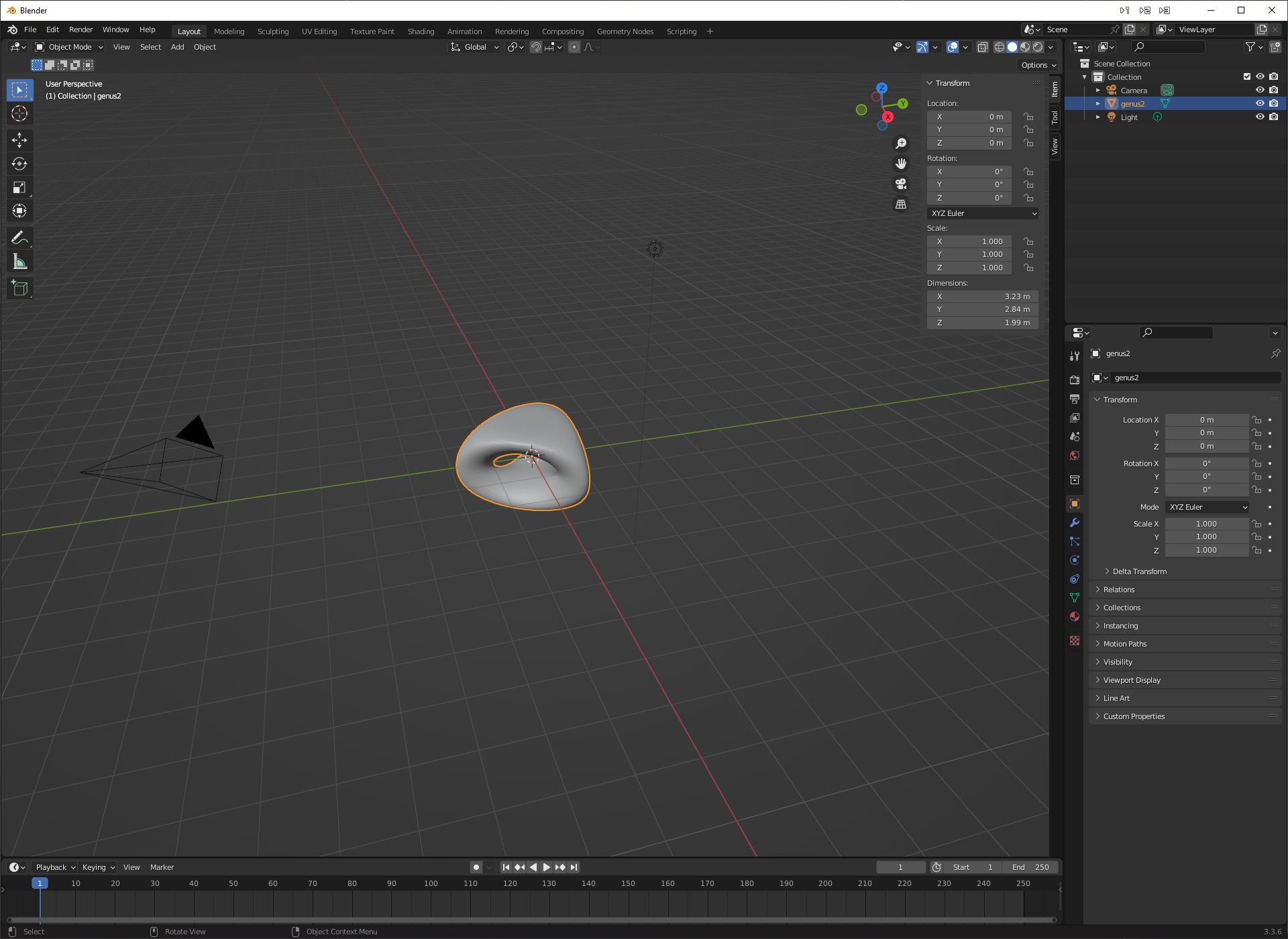
Select the file and click on Import PLY. You should now see something
similar as to the image below.
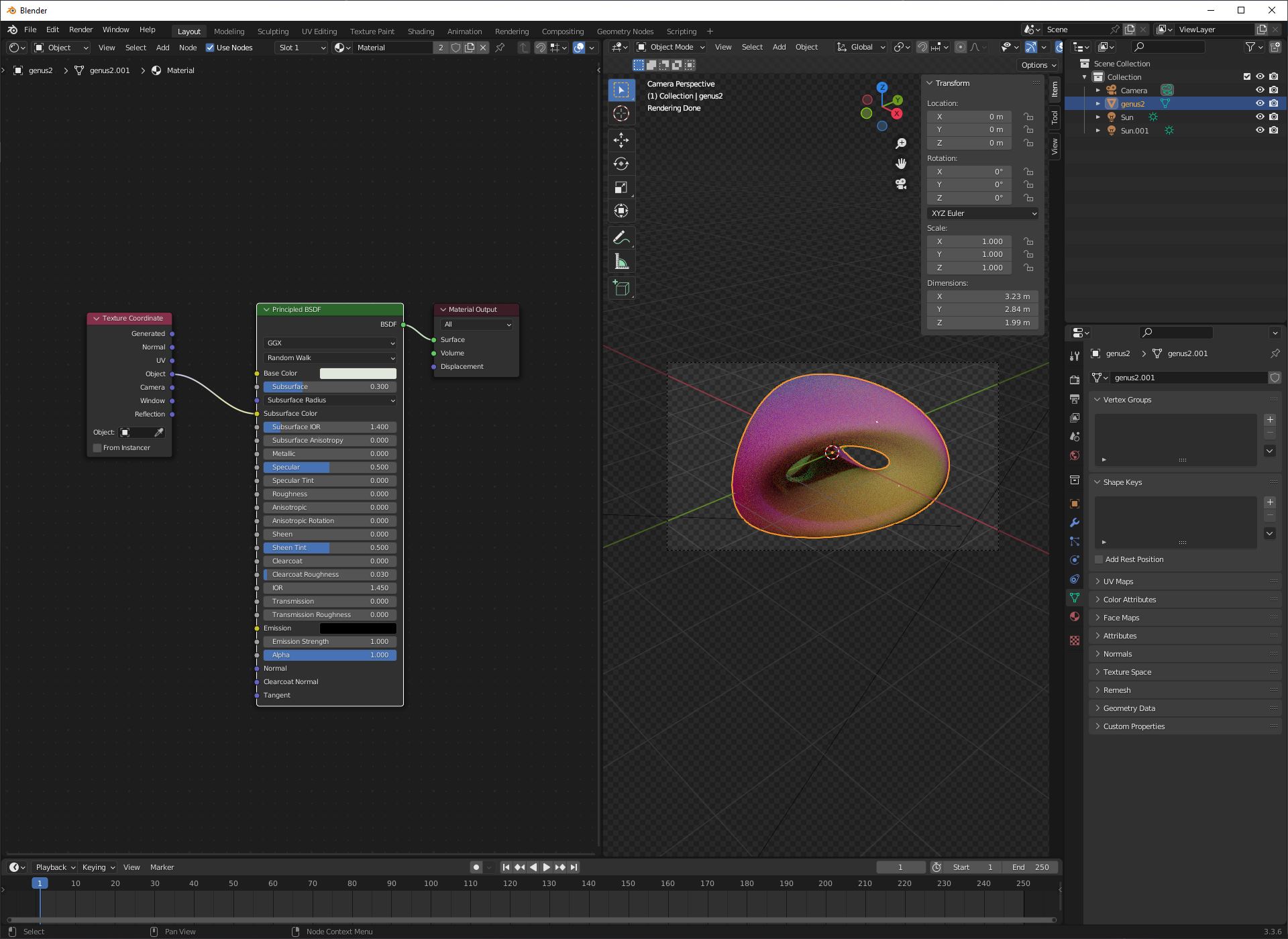
Finally, we assign a material to the object, tune the camera to bring the object fully into view, set the color of the background to black, add two sun-type light sources and set the film to transparent. For the material, we have used the settings as can be seen in the figure below.
The only step that remains is to render the image, which will give the image as shown at the start of this section.
Benzene highest occupied molecular orbital
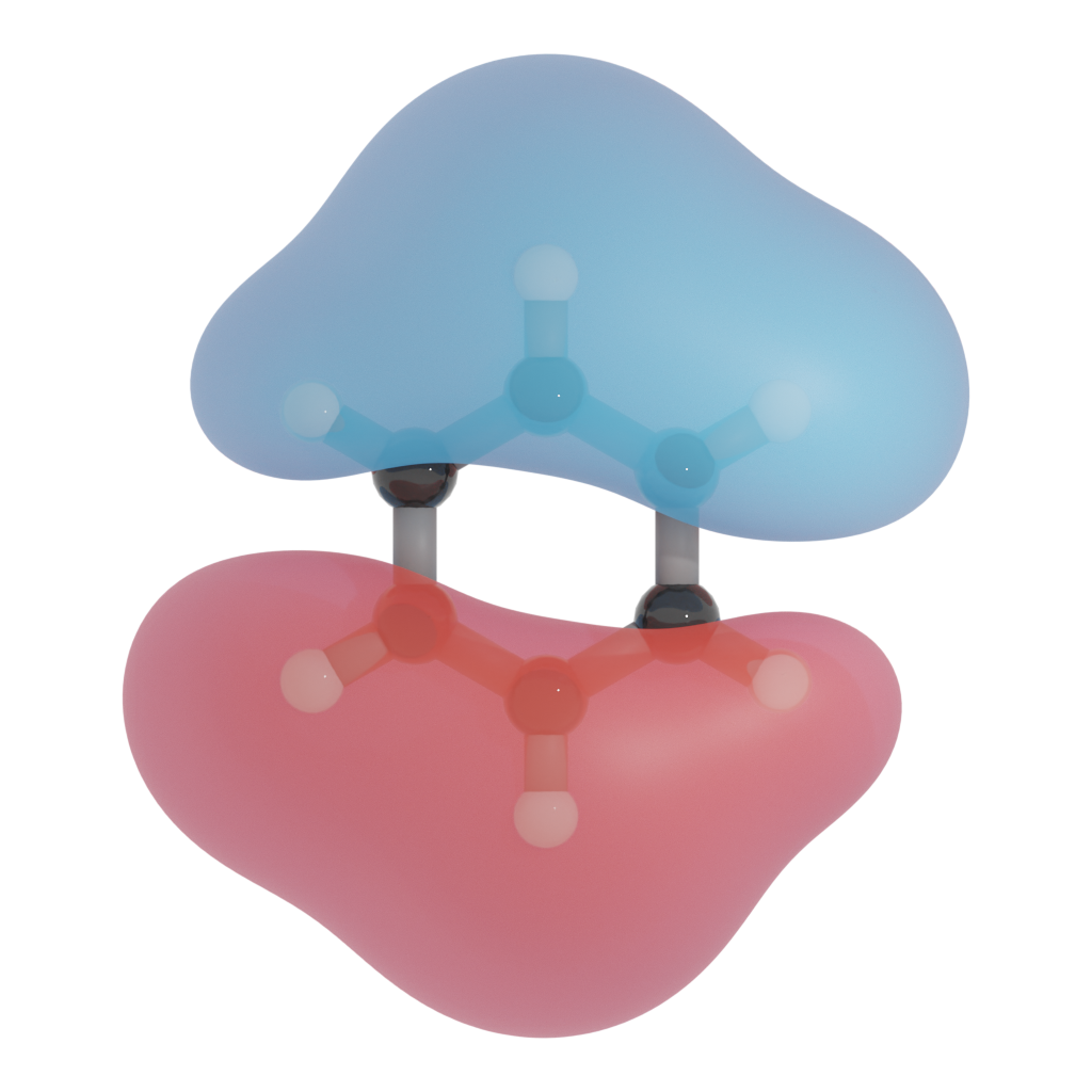
In this tutorial, we will be reproducing the Figure as shown below.
To generate the scalar field, run:
./den2obj -g benzene_homo -o benzene_homo.d2o
Next, the isosurface is generated. An isovalue of 0.03 is chosen. Because
molecular orbital have positive and negative lobes, we use the -d tag
to create both isosurfaces. Furthermore, we center the object by defining
-c and we explicitly ask to use the marching tetrahedra algorithm
via --algo marching-tetrahedra:
./den2obj -i benzene_homo.d2o -o benzene_homo.ply -v 0.03 -c -d --algo marching-tetrahedra
The following output (or similar) is generated:
--------------------------------------------------------------
Executing DEN2OBJ v.1.1.0
Author:  Ivo Filot <i.a.w.filot@tue.nl>
Website: https://den2obj.imc-tue.nl
Github:  https://github.com/ifilot/den2obj
--------------------------------------------------------------
Opening benzene_homo.d2o as D2O binary file
Recognizing floating point size: 4 bytes.
Reading 11415368 bytes from file.
Building LZMA decompressor
Decompressed data
Done reading D2O binary file
Read 3375000 values.
Using isovalue: 0.03
Lowest value in scalar field: -0.25383
Highest value in scalar field: 0.25383
Calculating normal vectors using two-point stencil
Centering structure
Writing mesh as Standford Triangle Format file (.ply).
Writing as Stanford (.ply) file: benzene_homo_pos.ply (4560.3kb).
Identified 59512 faces.
Calculating normal vectors using two-point stencil
Centering structure
Writing mesh as Standford Triangle Format file (.ply).
Writing as Stanford (.ply) file: benzene_homo_neg.ply (1454.4kb).
-------------------------------------------------------------------------------
Done in 2.17096 seconds.
Observe that two isosurfaces are created and stored as .ply files:
benzene_homo_pos.ply
benzene_homo_neg.ply
Importing these two files in Blender gives us the following result
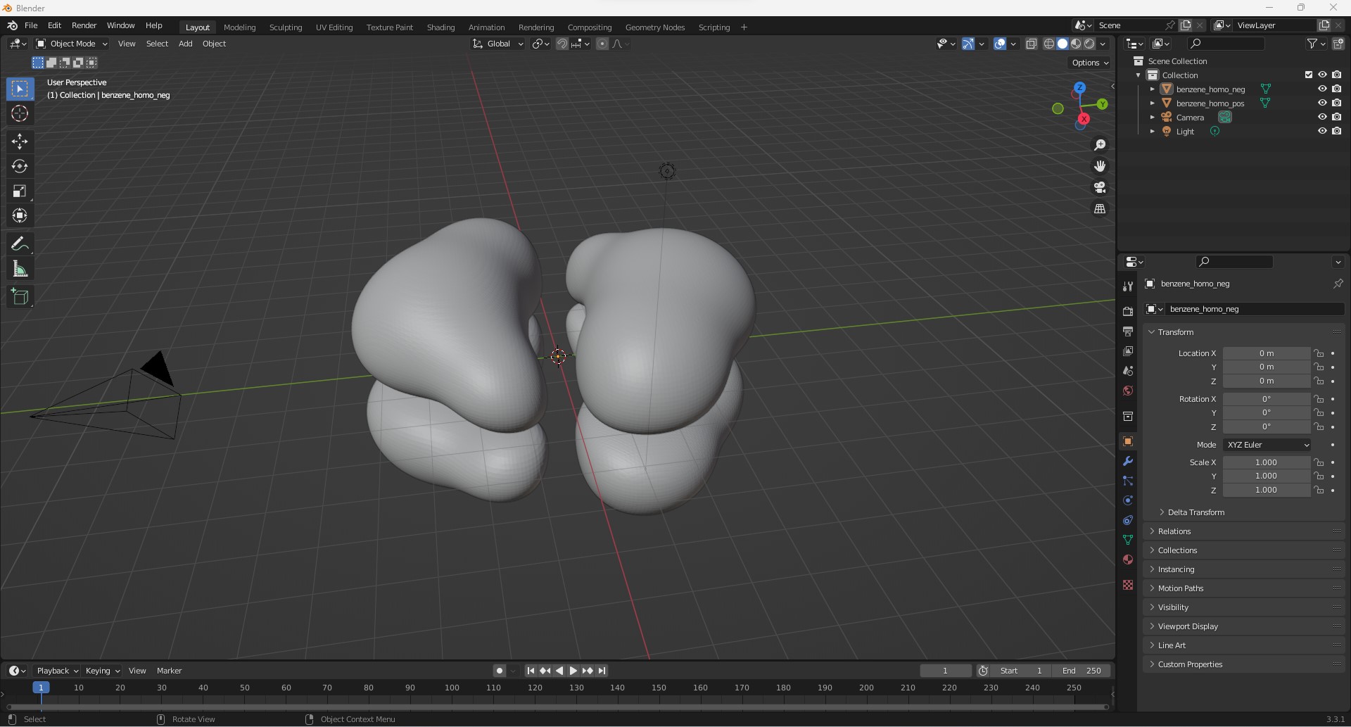
Of course, this result is rather blend and we would like to add the positions of the carbon and hydrogen atoms and the bonds between them. For this, we are going to use the hardcoded Python script as shown below which we can readily execute in Blender
import bpy
import numpy as np

def main():
    # define molecule
    mol = []

    mol.append(['C',  0.0000000015, -1.3868467444, 0.0000000000])
    mol.append(['C',  1.2010445126, -0.6934233709, 0.0000000000])
    mol.append(['C',  1.2010445111,  0.6934233735, 0.0000000000])
    mol.append(['C', -0.0000000015,  1.3868467444, 0.0000000000])
    mol.append(['C', -1.2010445126,  0.6934233709, 0.0000000000])
    mol.append(['C', -1.2010445111, -0.6934233735, 0.0000000000])
    mol.append(['H',  0.0000000027, -2.4694205285, 0.0000000000])
    mol.append(['H',  2.1385809117, -1.2347102619, 0.0000000000])
    mol.append(['H',  2.1385809090,  1.2347102666, 0.0000000000])
    mol.append(['H', -0.0000000027,  2.4694205285, 0.0000000000])
    mol.append(['H', -2.1385809117,  1.2347102619, 0.0000000000])
    mol.append(['H', -2.1385809090, -1.2347102666, 0.0000000000])

    build_atoms(mol)
    build_bonds(mol)

def build_atoms(molecule):
    for i,at in enumerate(molecule):
        sc = 0.4 if at[0] == 'C' else 0.3
        obj = bpy.ops.mesh.primitive_ico_sphere_add(radius=sc,
                                                    enter_editmode=False,
                                                    align='WORLD',
                                                    location=(at[1], at[2], at[3]),
                                                    scale=(1, 1, 1),
                                                    subdivisions=3)
        bpy.context.selected_objects[0].name = at[0] + str(i+1)
        bpy.ops.object.shade_smooth()

def build_bonds(molecule):
    z = np.array([0,0,1])
    for i,at1 in enumerate(molecule):
        p1 = np.array([at1[1], at1[2], at1[3]])
        for j,at2 in enumerate(molecule[i+1:]):
            p2 = np.array([at2[1], at2[2], at2[3]])
            d = np.linalg.norm(p1-p2)

            if d < 1.5:
                ctr = (p1 + p2) / 2
                angle = np.arccos(np.dot(z, (p2-p1) / d))
                axis = np.cross(z, (p2-p1) / d)
                axis /= np.linalg.norm(axis)

                bpy.ops.mesh.primitive_cylinder_add(radius=0.2,
                                                    depth=1,
                                                    enter_editmode=False,
                                                    align='WORLD',
                                                    location=(ctr[0], ctr[1], ctr[2]),
                                                    scale=(1, 1, 1))
                bpy.context.object.rotation_mode = 'AXIS_ANGLE'
                bpy.context.object.rotation_axis_angle[0] = angle
                bpy.context.object.rotation_axis_angle[1:4] = axis
                bpy.context.selected_objects[0].name = 'bond' + str(i+1) + '-' + str(j+1)
                bpy.ops.object.shade_smooth()


if __name__ == '__main__':
    main()
This will generate all the atoms and bonds between them. Next, materials are assigned to all atoms and bonds and the final result looks as seen in the image below.
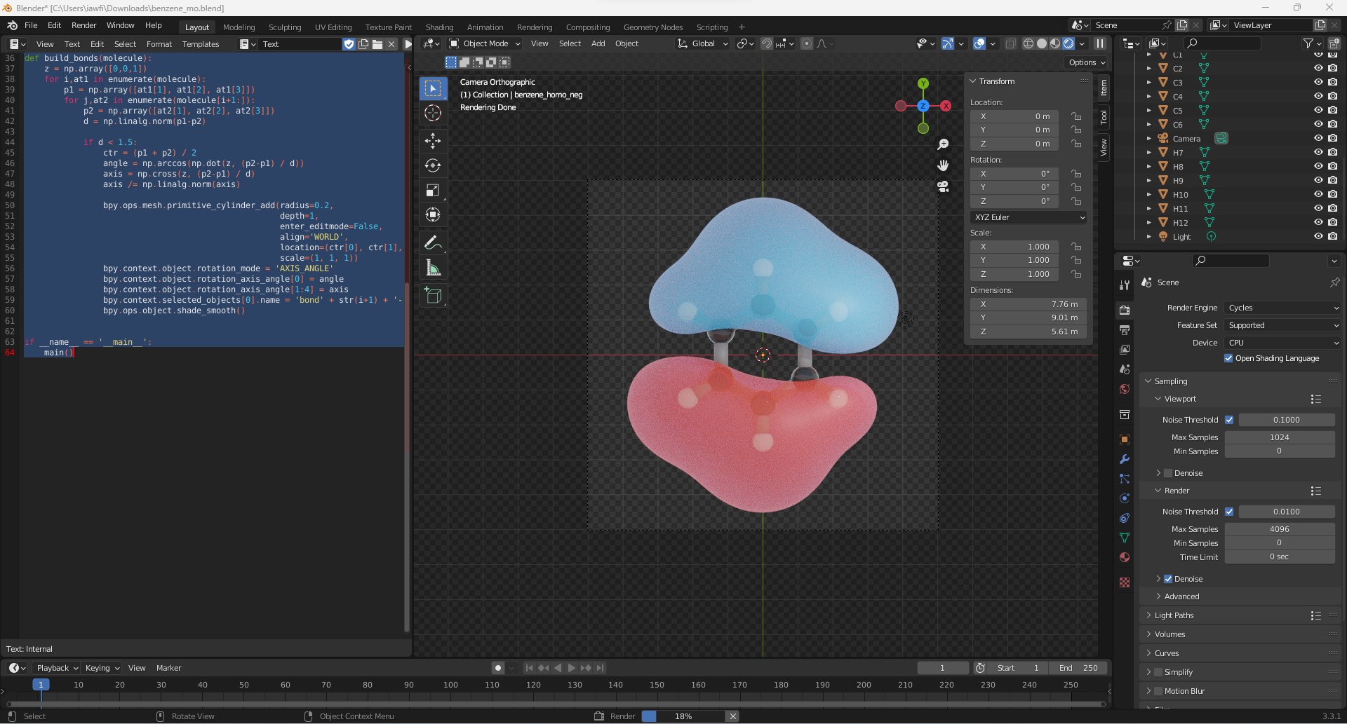
Finally, we can render the scene to create a nice picture of the molecular orbital.